Difference between revisions of "ChtMultiRegionFoam"
(→Coupling between Fluid and Solid) |
(→Equations) |
||
| Line 7: | Line 7: | ||
For each region defined as fluid, the according equation for the fluid is solved and the same is done | For each region defined as fluid, the according equation for the fluid is solved and the same is done | ||
| − | for each solid region. The regions are coupled by a thermal boundary condition. | + | for each solid region. The regions are coupled by a thermal boundary condition. A short description of |
the solver can be found also in <ref> EL ABBASSIA, M.; LAHAYE, D. J. P.; VUIK, C. MODELLING TURBULENT COMBUSTION COUPLED WITH CONJUGATE HEAT TRANSFER IN OPENFOAM.</ref> | the solver can be found also in <ref> EL ABBASSIA, M.; LAHAYE, D. J. P.; VUIK, C. MODELLING TURBULENT COMBUSTION COUPLED WITH CONJUGATE HEAT TRANSFER IN OPENFOAM.</ref> | ||
===Equations Fluid=== | ===Equations Fluid=== | ||
| − | For each fluid region the compressible Navier Stokes equation are solved. | + | For each fluid region the compressible Navier Stokes equation are solved. The solver used to solve the |
| + | fluid equations is a pressure bases solver. That means that a pressure equation (similar to the pressure equation used in an incompressible solver) | ||
| + | is used to establish the connection between the momentum and the continuity equation. The algorithm to advance the solution in time is the following: | ||
| + | |||
| + | 1. Update the density with the help of the continuity equation | ||
| + | |||
| + | 2. Solve the momentum equation | ||
| + | |||
| + | 3. Solve the spices transport equation | ||
| + | |||
| + | 4. Solve the energy equation | ||
| + | |||
| + | 5. Solve the pressure equation to ensure mass conservation | ||
| + | |||
| + | |||
| + | The source code can be found in solveFluid.H | ||
| + | |||
| + | <br><cpp> | ||
| + | |||
| + | if (pimple.frozenFlow()) | ||
| + | { | ||
| + | #include "EEqn.H" | ||
| + | } | ||
| + | else | ||
| + | { | ||
| + | if (!mesh.steady() && pimples.nCorrPimple() <= 1) | ||
| + | { | ||
| + | #include "rhoEqn.H" | ||
| + | } | ||
| + | |||
| + | #include "UEqn.H" | ||
| + | #include "YEqn.H" | ||
| + | #include "EEqn.H" | ||
| + | |||
| + | // --- PISO loop | ||
| + | while (pimple.correct()) | ||
| + | { | ||
| + | #include "pEqn.H" | ||
| + | } | ||
| + | |||
| + | if (pimples.pimpleTurbCorr(i)) | ||
| + | { | ||
| + | turbulence.correct(); | ||
| + | } | ||
| + | |||
| + | if (!mesh.steady() && pimples.finalIter()) | ||
| + | { | ||
| + | rho = thermo.rho(); | ||
| + | } | ||
| + | } | ||
| + | |||
| + | </cpp><br> | ||
| + | |||
====Mass conservation==== | ====Mass conservation==== | ||
Revision as of 17:26, 3 December 2018
ChtMultiRegionFoam
   Solver for steady or transient fluid flow and solid heat conduction, with
   conjugate heat transfer between regions, buoyancy effects, turbulence,
   reactions and radiation modelling.
Contents
1 Equations
For each region defined as fluid, the according equation for the fluid is solved and the same is done for each solid region. The regions are coupled by a thermal boundary condition. A short description of the solver can be found also in [1]
1.1 Equations Fluid
For each fluid region the compressible Navier Stokes equation are solved. The solver used to solve the fluid equations is a pressure bases solver. That means that a pressure equation (similar to the pressure equation used in an incompressible solver) is used to establish the connection between the momentum and the continuity equation. The algorithm to advance the solution in time is the following:
1. Update the density with the help of the continuity equation
2. Solve the momentum equation
3. Solve the spices transport equation
4. Solve the energy equation
5. Solve the pressure equation to ensure mass conservation
The source code can be found in solveFluid.H
if (pimple.frozenFlow())
{
    #include "EEqn.H"
}
else
{
    if (!mesh.steady() && pimples.nCorrPimple() <= 1)
    {
        #include "rhoEqn.H"
    }

    #include "UEqn.H"
    #include "YEqn.H"
    #include "EEqn.H"

    // --- PISO loop
    while (pimple.correct())
    {
        #include "pEqn.H"
    }

    if (pimples.pimpleTurbCorr(i))
    {
        turbulence.correct();
    }

    if (!mesh.steady() && pimples.finalIter())
    {
        rho = thermo.rho();
    }
}
1.1.1 Mass conservation
The variable-density continuity equation is
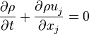 | (1) |
The source code can be found in src/finiteVolume/cfdTools/compressible/rhoEqn.H:
{
    fvScalarMatrix rhoEqn
    (
        fvm::ddt(rho)
      + fvc::div(phi)
      ==
        fvOptions(rho)
    );

    fvOptions.constrain(rhoEqn);

    rhoEqn.solve();

    fvOptions.correct(rho);
}
1.1.2 Momentum conservation
 | (2) |
 represent the velocity,
  the gravitational acceleration,
 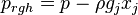 the pressure minus the hydrostatic pressure and
 and
and  are the viscose and turbulent stresses.
The source code can be found in Ueqn.H:
    // Solve the Momentum equation

    MRF.correctBoundaryVelocity(U);

    tmp<fvVectorMatrix> tUEqn
    (
        fvm::ddt(rho, U) + fvm::div(phi, U)
      + MRF.DDt(rho, U)
      + turbulence.divDevRhoReff(U)
     ==
        fvOptions(rho, U)
    );
    fvVectorMatrix& UEqn = tUEqn.ref();

    UEqn.relax();

    fvOptions.constrain(UEqn);

    if (pimple.momentumPredictor())
    {
        solve
        (
            UEqn
         ==
            fvc::reconstruct
            (
                (
                  - ghf*fvc::snGrad(rho)
                  - fvc::snGrad(p_rgh)
                )*mesh.magSf()
            )
        );

        fvOptions.correct(U);
        K = 0.5*magSqr(U);
    }

    fvOptions.correct(U);
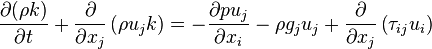
1.1.3 Energy conservation
The energy equation can be found in: https://cfd.direct/openfoam/energy-equation/
The total energy of a fluid element can be seen as the sum of kinetic energy  and internal energy
  .
The rate of change of the kinetic energy within a fluid element is the work done on this fluid element by the viscous forces, the pressure and eternal volume forces like the gravity:
.
The rate of change of the kinetic energy within a fluid element is the work done on this fluid element by the viscous forces, the pressure and eternal volume forces like the gravity:
 | (3) |
The rate of change of the internal energy of a fluid element is the heat transferred to this fluid element by diffusion and turbulence  plus the
heat source term
plus the
heat source term  plus the heat source by radiation
  :
:
 | (4) |
The change rate of the total energy is the sum of the above two equations:
 | (5) |
Instead of the internal energy there is also the option to solve the equation for the enthalpy 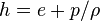 :
:
 | (5) |
The source code can be found in EEqn.H:
{
    volScalarField& he = thermo.he();

    fvScalarMatrix EEqn
    (
        fvm::ddt(rho, he) + fvm::div(phi, he)
      + fvc::ddt(rho, K) + fvc::div(phi, K)
      + (
            he.name() == "e"
          ? fvc::div
            (
                fvc::absolute(phi/fvc::interpolate(rho), U),
                p,
                "div(phiv,p)"
            )
          : -dpdt
        )
      - fvm::laplacian(turbulence.alphaEff(), he)
     ==
        rho*(U&g)
      + rad.Sh(thermo, he)
      + Qdot
      + fvOptions(rho, he)
    );

    EEqn.relax();

    fvOptions.constrain(EEqn);

    EEqn.solve();

    fvOptions.correct(he);

    thermo.correct();
    rad.correct();

    Info<< "Min/max T:" << min(thermo.T()).value() << ' '
        << max(thermo.T()).value() << endl;
}
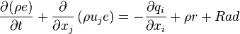
1.1.4 Species conservation
In order to account for the chemical reactions occurring between different chemical species a conservation equation for each species k has to be solved:
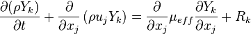 | (6) |
 is the reaction rate of the species k.
The source code can be found in YEqn.H:
tmp<fv::convectionScheme<scalar>> mvConvection(nullptr);

if (Y.size())
{
    mvConvection = tmp<fv::convectionScheme<scalar>>
    (
        fv::convectionScheme<scalar>::New
        (
            mesh,
            fields,
            phi,
            mesh.divScheme("div(phi,Yi_h)")
        )
    );
}

{
    reaction.correct();
    Qdot = reaction.Qdot();
    volScalarField Yt
    (
        IOobject("Yt", runTime.timeName(), mesh),
        mesh,
        dimensionedScalar("Yt", dimless, 0)
    );

    forAll(Y, i)
    {
        if (i != inertIndex && composition.active(i))
        {
            volScalarField& Yi = Y[i];

            fvScalarMatrix YiEqn
            (
                fvm::ddt(rho, Yi)
              + mvConvection->fvmDiv(phi, Yi)
              - fvm::laplacian(turbulence.muEff(), Yi)
             ==
                reaction.R(Yi)
              + fvOptions(rho, Yi)
            );

            YiEqn.relax();

            fvOptions.constrain(YiEqn);

            YiEqn.solve(mesh.solver("Yi"));

            fvOptions.correct(Yi);

            Yi.max(0.0);
            Yt += Yi;
        }
    }

    if (Y.size())
    {
        Y[inertIndex] = scalar(1) - Yt;
        Y[inertIndex].max(0.0);
    }
}
1.2 Equations Solid
For the solid regions only the energy equation has to be solved. The energy equation states that the temporal change of enthalpy of the solid is equal to the divergence of the heat conducted through the solid:
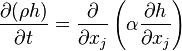 | (7) |
 is the specific enthalpy,
  the density and
  is the thermal
diffusivity which is defined as the ratio between the thermal conductivity
is the thermal
diffusivity which is defined as the ratio between the thermal conductivity  and the specific heat capacity
 . Note that can be also anisotropic.
The source code can be found in solveSolid.H:
{
    while (pimple.correctNonOrthogonal())
    {
        fvScalarMatrix hEqn
        (
            fvm::ddt(betav*rho, h)
          - (
                thermo.isotropic()
              ? fvm::laplacian(betav*thermo.alpha(), h, "laplacian(alpha,h)")
              : fvm::laplacian(betav*taniAlpha(), h, "laplacian(alpha,h)")
            )
          ==
            fvOptions(rho, h)
        );

        hEqn.relax();

        fvOptions.constrain(hEqn);

        hEqn.solve(mesh.solver(h.select(pimples.finalIter())));

        fvOptions.correct(h);


thermo.correct();

Info<< "Min/max T:" << min(thermo.T()).value() << ' '
    << max(thermo.T()).value() << endl;
1.3 Coupling between Fluid and Solid
A good explanation of the coupling between fluid and solid can be found in https://www.cfd-online.com/Forums/openfoam-solving/143571-understanding-temperature-coupling-bcs.html.
At the interface between solid s and fluid f the temperature T for both phases that to be the same:
 | (8) |
Furthermore the heat flux entering one region at one side of the interphase should be equal to the heat flux leaving the other region on the other side of the domain:
 | (9) |
If we neglect radiation the above expression can be written as:
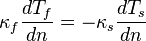 | (10) |
 represents the direction normal to the wall.
  and
and
 are the thermal conductivity of the fluid and solid, respectively.
The source code of the above boundary condition can be found in src/TurbulenceModels/compressible/turbulentFluidThermoModels/derivedFvPatchFields/turbulentTemperatureCoupledBaffleMixed/turbulentTemperatureCoupledBaffleMixedFvPatchScalarField.C
void turbulentTemperatureCoupledBaffleMixedFvPatchScalarField::updateCoeffs()
 {
     if (updated())
     {
         return;
     }

     // Since we're inside initEvaluate/evaluate there might be processor
     // comms underway. Change the tag we use.
     int oldTag = UPstream::msgType();
     UPstream::msgType() = oldTag+1;

     // Get the coupling information from the mappedPatchBase
     const mappedPatchBase& mpp =
         refCast<const mappedPatchBase>(patch().patch());
     const polyMesh& nbrMesh = mpp.sampleMesh();
     const label samplePatchi = mpp.samplePolyPatch().index();
     const fvPatch& nbrPatch =
         refCast<const fvMesh>(nbrMesh).boundary()[samplePatchi];

     // Calculate the temperature by harmonic averaging
     // ~~~~~~~~~~~~~~~~~~~~~~~~~~~~~~~~~~~~~~~~~~~~~~~

     const turbulentTemperatureCoupledBaffleMixedFvPatchScalarField& nbrField =
     refCast
     <
         const turbulentTemperatureCoupledBaffleMixedFvPatchScalarField
     >
     (
         nbrPatch.lookupPatchField<volScalarField, scalar>
         (
             TnbrName_
         )
     );

     // Swap to obtain full local values of neighbour internal field
     tmp<scalarField> nbrIntFld(new scalarField(nbrField.size(), 0.0));
     tmp<scalarField> nbrKDelta(new scalarField(nbrField.size(), 0.0));

     if (contactRes_ == 0.0)
     {
         nbrIntFld.ref() = nbrField.patchInternalField();
         nbrKDelta.ref() = nbrField.kappa(nbrField)*nbrPatch.deltaCoeffs();
     }
     else
     {
         nbrIntFld.ref() = nbrField;
         nbrKDelta.ref() = contactRes_;
     }

     mpp.distribute(nbrIntFld.ref());
     mpp.distribute(nbrKDelta.ref());

     tmp<scalarField> myKDelta = kappa(*this)*patch().deltaCoeffs();


     // Both sides agree on
     // - temperature : (myKDelta*fld + nbrKDelta*nbrFld)/(myKDelta+nbrKDelta)
     // - gradient    : (temperature-fld)*delta
     // We've got a degree of freedom in how to implement this in a mixed bc.
     // (what gradient, what fixedValue and mixing coefficient)
     // Two reasonable choices:
     // 1. specify above temperature on one side (preferentially the high side)
     //    and above gradient on the other. So this will switch between pure
     //    fixedvalue and pure fixedgradient
     // 2. specify gradient and temperature such that the equations are the
     //    same on both sides. This leads to the choice of
     //    - refGradient = zero gradient
     //    - refValue = neighbour value
     //    - mixFraction = nbrKDelta / (nbrKDelta + myKDelta())

     this->refValue() = nbrIntFld();
     this->refGrad() = 0.0;
     this->valueFraction() = nbrKDelta()/(nbrKDelta() + myKDelta());

     mixedFvPatchScalarField::updateCoeffs();

     if (debug)
     {
         scalar Q = gSum(kappa(*this)*patch().magSf()*snGrad());

         Info<< patch().boundaryMesh().mesh().name() << ':'
             << patch().name() << ':'
             << this->internalField().name() << " <- "
             << nbrMesh.name() << ':'
             << nbrPatch.name() << ':'
             << this->internalField().name() << " :"
             << " heat transfer rate:" << Q
             << " walltemperature "
             << " min:" << gMin(*this)
             << " max:" << gMax(*this)
             << " avg:" << gAverage(*this)
             << endl;
     }

     // Restore tag
     UPstream::msgType() = oldTag;
 }
2 Source Code
3 References
- ↑ EL ABBASSIA, M.; LAHAYE, D. J. P.; VUIK, C. MODELLING TURBULENT COMBUSTION COUPLED WITH CONJUGATE HEAT TRANSFER IN OPENFOAM.